


Machine learning has become more accessible with the help of toolboxes like PyTorch, Keras, and scikit-learn. However, using these tools with caution is important to avoid common pitfalls. In this article, we'll explore some traps to watch out for and how to avoid them.
An example
As an example, consider an engineer who has developed a state-of-the-art machine called the NiceDevice. This machine is equipped with 2000 sensors and has a quality measure called the 'average deviation', which is better the closer it is to zero. To prevent the machine from failing, the engineer wants to predict the quality of the NiceDevice on the next day using sensor data from the current day.
The engineer has data from 1200 days and wants to train a neural network to make this prediction. The first important step in this process is to determine how to test the performance of the model. To do this, the engineer sets aside some test data that they don't feed to the algorithm, so that the neural network doesn't simply memorize the data.
To predict the ‘average deviation’ from the sensor data, we use Artificial Neural Networks (ANNs). ANNs are a machine learning technique whose architecture is inspired by the human brain and can be used to predict values based on training data. Similar to a human brain, a neural network has ‘neurons’ that are connected by ‘synapses’. Here we use a feed-forward neural network with different layers of interconnected neurons to form a neural network. Let’s understand it more deeply through a representation of a neural network.
Architecture of neural network
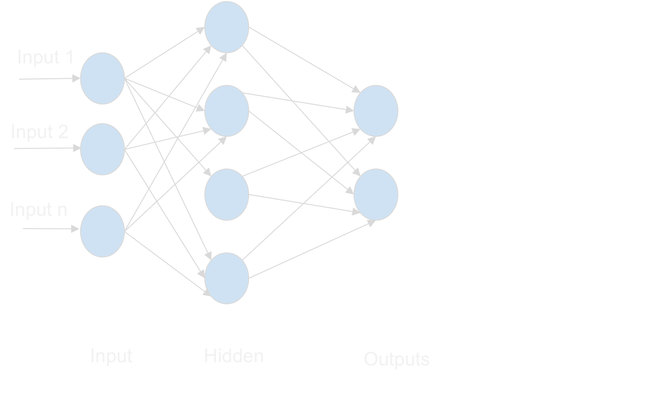
The first layer is the input layer; we fed several inputs (features) to the neural network. The second layer is the hidden layer which takes the input from the input layer multiplied by synaptic weights, sums them up and modifies them by an activation function. The activation of the hidden neuron h is computed by
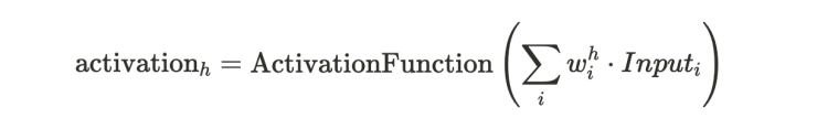
here, the synaptic weight wᵢʰ is the connection of the input neuron i with the hidden neuron h.
The final layer is the output layer, which does a similar processing as the hidden layer, this time with the activations from the hidden layer as an input. This is a very basic representation of ANN. However, in practice, we might have several inputs and several hidden layers, which then makes it a deep neural network, which is called ‘Deep Learning’.
Training of Neural Networks
In our case, we will train a simple neural network with a single hidden layer to predict the quality of the NiceDevice. The training process involves minimizing the mean squared error (MSE), which is a measure of the difference between the predicted and actual values. The MSE is calculated as the average of the squared differences between the predicted and target values and is given by the following formula:
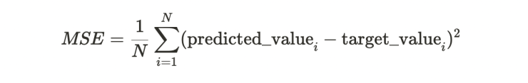
where N is the number of data points and Σ denotes the sum over all data points i.
Since the predicted value is actually the output of the neural network, the MSE is a function of the neural network weights. Training the neural network is basically minimizing the MSE with respect to these parameters by computing the derivative of the MSE and changing the neural network weights so that the MSE is minimized.
Here we use the scikit-learn¹ package in python to do this. We don’t actually have to bother computing derivatives and minimizing the function, but we just need to call fit. Or as we do it here partial_fit, which does a single update step.
In this code we use the MLPRegressor from scikit-learn, which is by default a feedforward neural network with a single hidden layer with 100 nodes. It is a regressor, as opposed to a classifier, since it is used to estimate a continuous number, while a classifier estimates discrete classes².
The MLPRegressor has a fit function, which we could directly use to fit the model in a single command (internally it does a loop over multiple update steps), however we want to see in more detail what happens to the error on the training set during training, therefore we explicitly write a loop over 200 training steps.
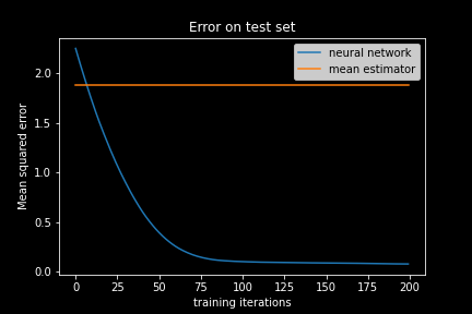
In each of these loops we randomly sample 200 data points from our training set (called a minibatch) and conduct a partial_fit, which means a single change in the weights of the neural network. After each update we compute the MSE error on the test set which we set aside.
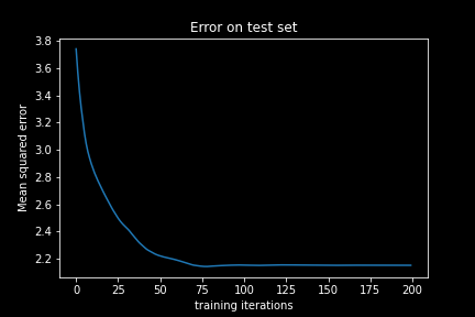
We see that the error on the test set does indeed decrease and then saturates. Well, it seems that our neural network learned something. Or wait, did it actually? The neural network is initialized with random weights, which leads to a high initial error. This error did decrease, but is the prediction quality really ‘good’? Did the neural network actually learn anything useful? How small must the MSE be in order to deduce that the neural network can meaningfully predict our target value, the ‘average deviation’?
Evaluating the trained Neural Network
To answer this question, let us consider a baseline estimator for the target value: the mean estimator, which is just taking the average of the target values in the training data set as our predicted value, independent of the sensor data.
The error for this estimator can be computed as

Which is nothing more than the variance of the target values.
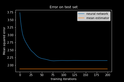
Here we have the orange line denoting the baseline MSE. It looks like that the mean estimator is actually better than the neural network! How embarrassing! A simple average is better than our complex machine learning algorithm that is inspired by the brain?
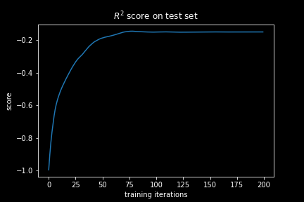
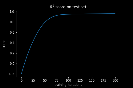
It is quite tempting when using machine learning to just look at the MSE to see how well the neural network is learning, since it is used as the error function that is minimized. However a more informative measure about the predictive performance of the neural network is the coefficient of determination, also known as the R² value, which is defined as

Basically, the MSE is normalized with the MSE of the mean estimator.
If the R² value is smaller than 0, then our estimator is worse than the mean estimator, if it is exactly 0 it is on par with it and if the R² is equal to 1 the estimator is perfect.
If we plot the R² for our neural network during the training we immediately see that while it is increasing, it saturates on a value below zero. Hence, it never really learns to make any meaningful prediction and is thus quite useless!
Making it actually work
So, what went wrong? Why is the neural network doing such a bad job?
To answer this question let us take a closer look at our data set, by plotting the sensor values on each day versus the average deviation on the following day for sensors 1-8.
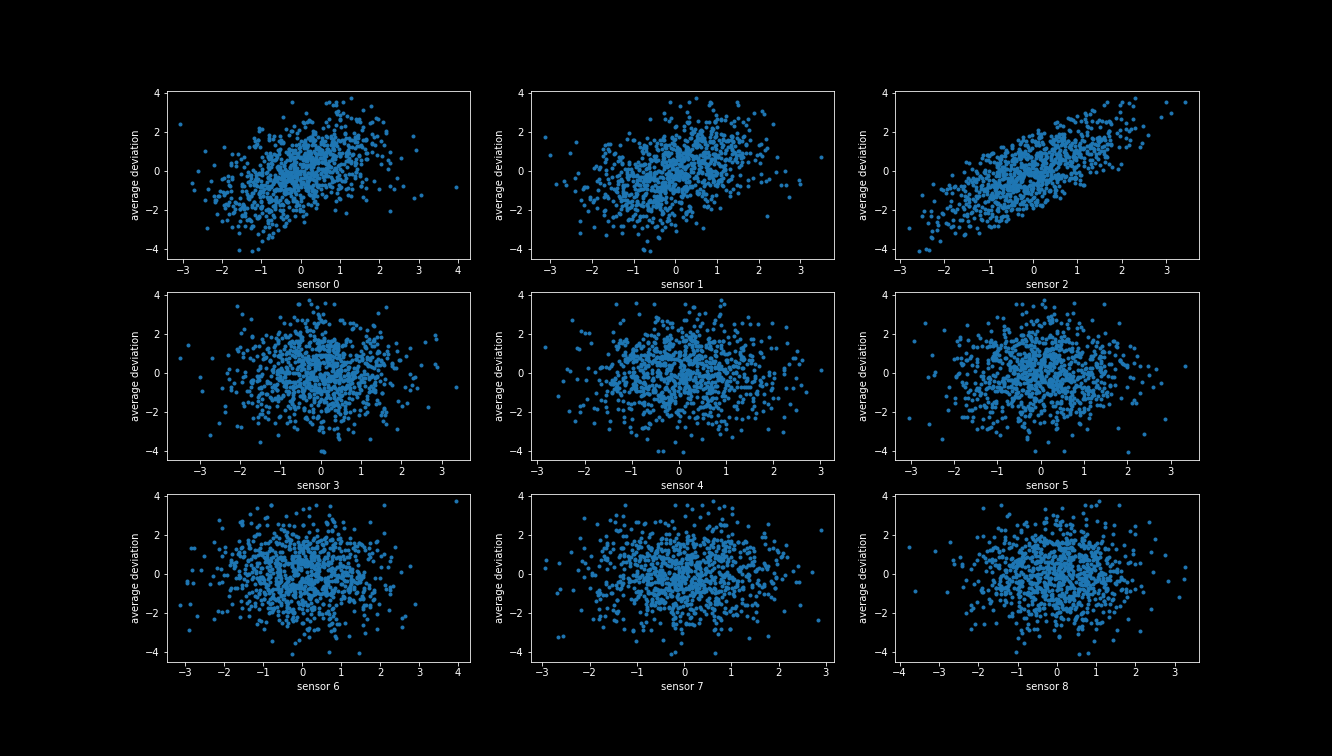
From these plots, we can see that there is a correlation between the first three sensors and target value, with the 3rd sensor having the clearest pattern. In the other sensors it does not look like there is any correlation. To verify this, we compute the correlation coefficients for each sensor (we only show the first 50 here).
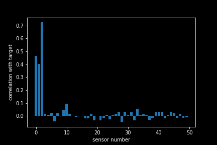
Indeed, it seems while there is a strong correlation of the sensors 1,2 and 3 with our target value, the other sensor seems not to strongly correlate with it³. It seems that by feeding all 550 sensors into our neural network, we have fed mostly noise and hardly any signal. Picking up this signal is like finding a needle in the haystack!
Let us try to make the task for our neural network a little easier, by only feeding it features that are correlating with the target value and see how it performs.
We can employ the SelectKBest feature selector from the scikit-learn package, to select only the top 3 features. We tell the selector to use the r_regression measure, which measures the Pearson correlation coefficient between the feature and the target, as we have done in our visualization.
feature_selector = SelectKBest(r_regression, k=3)X_train_selected = feature_selector.fit_transform(X_train, y_train)X_test_selected = feature_selector.transform(X_test)
After selecting the features we train the neural network again.
Now we see that the MSE dropped well below the baseline MSE of the mean estimator which is reflected in the R² value that is now saturating on a value close to 1. At this state, the neural network has actually learned something. Considering that we computed our score on a left out test set, we are assured that it did not only memorize the data points in the training data, but that it can as well generalize to new data.
Conclusion
Task accomplished! Our engineer can use this neural network to build a warning lamp into the NiceDevice that monitors and predicts a quality decay on the next day so that the machine can be maintained and not fail in production.
If you have enough data and the signal is not hard to find, you can get good performance even if you rely only on the MSE. However, as pointed out here, things can go wrong, and without considering statistical measures such as the coefficient of determination, low performance can go unnoticed. What has been your experience with this? Did you directly learn how to do it properly, or did you learn it the hard way?
Footnotes:
(1) For more complex tasks such as image recognition or natural language processing, more advanced tools such as PyTorch or Keras may be needed. However, for our simple neural network, scikit-learn provides a sufficient solution.
(2) When it comes to neural networks, there are some key differences between those designed for classification versus regression. Firstly, in a classification neural network, the final layer's output is typically transformed to fall within the range of 0 to 1, as this allows the network to output the probability of each potential class. Secondly, classification neural networks use a different type of error function, known as the logistic loss function. This function is better suited for identifying classification errors compared to the Mean Squared Error (MSE) function, which is typically used in regression neural networks to measure the deviation of a predicted output from a single target value.
(3) In a correlation plot, a large positive number indicates a positive correlation between two variables. This means that a high sensor value is likely to correspond with a high quality value. Conversely, a large negative number indicates a negative correlation between two variables. Small numbers, whether negative or positive, indicate no linear correlation between the variables. When there is no linear correlation, it suggests that the variables are unlikely to be useful as predictor features. However, it's important to note that non-linear correlations may still exist, although that topic is beyond the scope of this particular blog post.


